RPACT Survival Designs

Gernot Wassmer and Friedrich Pahlke

November 19, 2024

RPACT Survival Designs

The Situation

Assume we want to design a two-arm group sequential trial with a time to event endpoint where the summary measure of interest is the hazard ratio \(\omega\)

Suppose we wish to test

\[ H_0: \omega \geq 1 \text{ against } H_1: \omega < 1 \]

We require:

\(\alpha = 0.025\)
Power \(1 - \beta = 0.8\) at \(\omega = 0.6\)
Allocation ratio 1 : 1

Required Number of Events

Question 1

How many events would be required for a fixed sample size design?

library(rpact)
getSampleSizeSurvival(
    alpha = 0.025, 
    beta = 0.2, 
    hazardRatio = 0.6
) |> summary()

Sample size calculation for a survival endpoint

Fixed sample analysis, one-sided significance level 2.5%, power 80%. The results were calculated for a two-sample logrank test, H0: hazard ratio = 1, H1: hazard ratio = 0.6, control pi(2) = 0.2, event time = 12, accrual time = 12, accrual intensity = 62.1, follow-up time = 6.

Stage	Fixed
Stage level (one-sided)	0.0250
Efficacy boundary (z-value scale)	1.960
Efficacy boundary (t)	0.700
Number of subjects	745.0
Number of events	120.3
Analysis time	18.00
Expected study duration under H1	18.00

Legend:

(t): treatment effect scale

Required Number Of Subjects

Obviously, some default parameters were used to derive the required number of subjects

getSampleSizeSurvival(hazardRatio = 0.6) |> print()

Design plan parameters and output for survival data

Design parameters

Critical values: 1.960
Significance level: 0.0250
Type II error rate: 0.2000
Test: one-sided

User defined parameters

Hazard ratio: 0.600

Default parameters

Theta H0: 1
Type of computation: Schoenfeld
Assumed control rate: 0.200
Planned allocation ratio: 1
Event time: 12
Accrual time: 12.00
kappa: 1
Follow up time: 6.00
Drop-out rate (1): 0.000
Drop-out rate (2): 0.000
Drop-out time: 12.00

Sample size and output

Direction upper: FALSE
Assumed treatment rate: 0.125
median(1): 62.1
median(2): 37.3
lambda(1): 0.0112
lambda(2): 0.0186
Number of events: 120.3
Accrual intensity: 62.1
Number of events fixed: 120.3
Number of subjects fixed: 745
Number of subjects fixed (1): 372.5
Number of subjects fixed (2): 372.5
Analysis time: 18.00
Study duration: 18.00
Critical values (treatment effect scale): 0.700

Legend

(i): values of treatment arm i

Required Number Of Subjects

For the survival time distributions, we assume:

Median survival on the control arm is 1 year.
Exponential survival distribution.

Question 2

What is the sample size (number of subjects) for a fixed sample size design if the recruitment lasts 3 years and the (additional) follow-up time lasts 2 years, i.e., it is planned to conduct the study in 5 years?

getSampleSizeSurvival(
    alpha = 0.025, 
    beta = 0.2, 
    hazardRatio = 0.6, 
    median2 = 1, 
    accrualTime = 3,
    followUpTime = 2
) |> summary()

Required Number Of Subjects

Sample size calculation for a survival endpoint

Fixed sample analysis, one-sided significance level 2.5%, power 80%. The results were calculated for a two-sample logrank test, H0: hazard ratio = 1, H1: hazard ratio = 0.6, control median(2) = 1, accrual time = 3, accrual intensity = 48.7, follow-up time = 2.

Stage	Fixed
Stage level (one-sided)	0.0250
Efficacy boundary (z-value scale)	1.960
Efficacy boundary (t)	0.700
Number of subjects	146.2
Number of events	120.3
Analysis time	5.00
Expected study duration under H1	5.00

Legend:

(t): treatment effect scale

For recruitment assumptions, we assume:

It is possible to recruit 50 subjects per year at a uniform rate.
Recruitment lasts 3 years.
I.e., slightly higher number of available subjects.

Follow-up time needs to be calculated

Question 3

What is the expected study duration for a fixed sample size design?

getSampleSizeSurvival(
    alpha = 0.025, 
    beta = 0.2, 
    hazardRatio = 0.6, 
    median2 = 1, 
    accrualTime = c(0, 3),
    accrualIntensity = 50
) |> summary()

Sample size calculation for a survival endpoint

Fixed sample analysis, one-sided significance level 2.5%, power 80%. The results were calculated for a two-sample logrank test, H0: hazard ratio = 1, H1: hazard ratio = 0.6, control median(2) = 1, accrual time = 3, accrual intensity = 50.

Stage	Fixed
Stage level (one-sided)	0.0250
Efficacy boundary (z-value scale)	1.960
Efficacy boundary (t)	0.700
Number of subjects	150.0
Number of events	120.3
Analysis time	4.78
Expected study duration under H1	4.78

Legend:

(t): treatment effect scale

Question 4

Suppose recruitment lasts 3.5 years instead of 3 years. What would be the expected study duration for a fixed sample size design?

getSampleSizeSurvival(
    alpha = 0.025, 
    beta = 0.2, 
    hazardRatio = 0.6, 
    median2 = 1, 
    accrualTime = c(0, 3.5),
    accrualIntensity = 50
) |> summary()

Sample size calculation for a survival endpoint

Fixed sample analysis, one-sided significance level 2.5%, power 80%. The results were calculated for a two-sample logrank test, H0: hazard ratio = 1, H1: hazard ratio = 0.6, control median(2) = 1, accrual time = 3.5, accrual intensity = 50.

Stage	Fixed
Stage level (one-sided)	0.0250
Efficacy boundary (z-value scale)	1.960
Efficacy boundary (t)	0.700
Number of subjects	175.0
Number of events	120.3
Analysis time	4.20
Expected study duration under H1	4.20

Legend:

(t): treatment effect scale

Adding An Interim Analysis

We wish to add an interim analysis for efficacy. The interim should happen after approximately half the required number of events. An O’Brien-Fleming type alpha-spending function will be used. No futility analysis is considered (for now).

design <- getDesignGroupSequential(
    typeOfDesign = "asOF", 
    kMax = 2, 
    alpha = 0.025, 
    beta = 0.2
)

Question 5

Using the same design assumptions as above with a recruitment period of 3.5 years, perform the sample size calculation.

getSampleSizeSurvival(
    design = design,
    hazardRatio = 0.6, 
    median2 = 1, 
    accrualTime = c(0, 3.5),
    accrualIntensity = 50
) |> summary()

Adding An Interim Analysis

Sample size calculation for a survival endpoint

Sequential analysis with a maximum of 2 looks (group sequential design), one-sided overall significance level 2.5%, power 80%. The results were calculated for a two-sample logrank test, H0: hazard ratio = 1, H1: hazard ratio = 0.6, control median(2) = 1, accrual time = 3.5, accrual intensity = 50.

Stage	1	2
Planned information rate	50%	100%
Cumulative alpha spent	0.0015	0.0250
Stage levels (one-sided)	0.0015	0.0245
Efficacy boundary (z-value scale)	2.963	1.969
Efficacy boundary (t)	0.466	0.699
Cumulative power	0.1641	0.8000
Number of subjects	130.3	175.0
Expected number of subjects under H1		167.7
Cumulative number of events	60.4	120.8
Expected number of events under H1		110.9
Analysis time	2.61	4.22
Expected study duration under H1		3.95
Exit probability for efficacy (under H0)	0.0015
Exit probability for efficacy (under H1)	0.1641

Legend:

(t): treatment effect scale

After how many events is the interim and final analysis to take place?
How long would it take to reach the required number of interim and final events according to the design assumptions?
What is the critical value for the hazard ratio at the interim and final analysis?
What is the expected study duration according to the design assumptions (i.e., under the alternative hypothesis)?
What is the expected number of subjects according to the design assumptions (i.e., under the alternative hypothesis)?
What is the expected number of events under the null hypothesis and under the alternative?

getSampleSizeSurvival(
    design = design,
    hazardRatio = 0.6, 
    median2 = 1, 
    accrualTime = c(0, 3.5),
    accrualIntensity = 50
) |> print()

Design plan parameters and output for survival data

Design parameters

Information rates: 0.500, 1.000
Critical values: 2.963, 1.969
Futility bounds (non-binding): -Inf
Cumulative alpha spending: 0.001525, 0.025000
Local one-sided significance levels: 0.001525, 0.024500
Significance level: 0.0250
Type II error rate: 0.2000
Test: one-sided

User defined parameters

median(2): 1.0
Hazard ratio: 0.600
Accrual time: 3.50
Accrual intensity: 50.0

Default parameters

Theta H0: 1
Type of computation: Schoenfeld
Planned allocation ratio: 1
kappa: 1
Drop-out rate (1): 0.000
Drop-out rate (2): 0.000
Drop-out time: 12.00

Sample size and output

Direction upper: FALSE
median(1): 1.7
lambda(1): 0.416
lambda(2): 0.693
Maximum number of subjects: 175
Maximum number of subjects (1): 87.5
Maximum number of subjects (2): 87.5
Number of subjects [1]: 130.3
Number of subjects [2]: 175
Maximum number of events: 120.8
Follow up time: 0.72
Reject per stage [1]: 0.1641
Reject per stage [2]: 0.6359
Early stop: 0.1641
Analysis time [1]: 2.61
Analysis time [2]: 4.22
Expected study duration: 3.95
Maximal study duration: 4.22
Cumulative number of events [1]: 60.4
Cumulative number of events [2]: 120.8
Expected number of events under H0: 120.7
Expected number of events under H0/H1: 119.3
Expected number of events under H1: 110.9
Expected number of subjects under H1: 167.7
Critical values (treatment effect scale) [1]: 0.466
Critical values (treatment effect scale) [2]: 0.699

Legend

(i): values of treatment arm i
[k]: values at stage k

Adding A Futility Boundary

Suppose at the time of the interim analysis we wish to add a futility stopping boundary.

A simple rule is considered: if the Z-statistic is above zero (where negative values of the Z-statistic indicate treatment benefit), then the trial is stopped for futility.

The rule is considered non-binding.

Question 6

Create a design object which includes this futility stopping rule.

designWithFutility <- getDesignGroupSequential(
    typeOfDesign = "asOF", 
    kMax = 2, 
    futilityBounds = 0,
    alpha = 0.025, 
    beta = 0.2
)

Use the function getPowerSurvival() to calculate the overall power when adding the futility boundary under the same design assumptions as above. Assume recruitment lasts for 3.5 years (50 subjects per year). Assume that the maximum number of events is 121. What is the the overall power? The expected study duration and number of subjects?

Direction of test statistic

Specify directionUpper = FALSE because power is directed towards hazard ratio < 1

getPowerSurvival(
    design = designWithFutility,
    hazardRatio = 0.6, 
    median2 = 1, 
    directionUpper = FALSE, 
    maxNumberOfEvents = 121,
    accrualTime = c(0, 3.5),
    accrualIntensity = 50
) |> summary()

Power calculation for a survival endpoint

Sequential analysis with a maximum of 2 looks (group sequential design), one-sided overall significance level 2.5%. The results were calculated for a two-sample logrank test, H0: hazard ratio = 1, power directed towards smaller values, H1: hazard ratio = 0.6, control median(2) = 1, maximum number of events = 121, accrual time = 3.5, accrual intensity = 50.

Stage	1	2
Planned information rate	50%	100%
Cumulative alpha spent	0.0015	0.0250
Stage levels (one-sided)	0.0015	0.0245
Efficacy boundary (z-value scale)	2.963	1.969
Futility boundary (z-value scale)	0
Efficacy boundary (t)	0.467	0.699
Futility boundary (t)	1.000
Cumulative power	0.1645	0.7977
Number of subjects	130.5	175.0
Expected number of subjects under H1		166.6
Cumulative number of events	60.5	121.0
Expected number of events under H1		109.6
Analysis time	2.61	4.22
Expected study duration under H1		3.92
Overall exit probability (under H0)	0.5015
Overall exit probability (under H1)	0.1880
Exit probability for efficacy (under H0)	0.0015
Exit probability for efficacy (under H1)	0.1645
Exit probability for futility (under H0)	0.5000
Exit probability for futility (under H1)	0.0235

Legend:

(t): treatment effect scale

What is the expected study duration and number of subjects under the null hypothesis?

getPowerSurvival(
    design = designWithFutility,
    hazardRatio = 1, 
    median2 = 1, 
    directionUpper = FALSE, 
    maxNumberOfEvents = 121,
    accrualTime = c(0, 3.5),
    accrualIntensity = 50
) |> summary()

Power calculation for a survival endpoint

Sequential analysis with a maximum of 2 looks (group sequential design), one-sided overall significance level 2.5%. The results were calculated for a two-sample logrank test, H0: hazard ratio = 1, power directed towards smaller values, H1: hazard ratio = 1, control median(2) = 1, maximum number of events = 121, accrual time = 3.5, accrual intensity = 50.

Stage	1	2
Planned information rate	50%	100%
Cumulative alpha spent	0.0015	0.0250
Stage levels (one-sided)	0.0015	0.0245
Efficacy boundary (z-value scale)	2.963	1.969
Futility boundary (z-value scale)	0
Efficacy boundary (t)	0.467	0.699
Futility boundary (t)	1.000
Cumulative power	0.0015	0.0247
Number of subjects	118.7	175.0
Expected number of subjects under H1		146.8
Cumulative number of events	60.5	121.0
Expected number of events under H1		90.7
Analysis time	2.37	3.78
Expected study duration under H1		3.08
Overall exit probability (under H0)	0.5015
Overall exit probability (under H1)	0.5015
Exit probability for efficacy (under H0)	0.0015
Exit probability for efficacy (under H1)	0.0015
Exit probability for futility (under H0)	0.5000
Exit probability for futility (under H1)	0.5000

Legend:

(t): treatment effect scale

Together:

getPowerSurvival(
    design = designWithFutility,
    hazardRatio = c(0.6, 1), 
    median2 = 1, 
    directionUpper = FALSE, 
    maxNumberOfEvents = 121,
    accrualTime = c(0, 3.5),
    accrualIntensity = 50
) |> summary()

Power calculation for a survival endpoint

Sequential analysis with a maximum of 2 looks (group sequential design), one-sided overall significance level 2.5%. The results were calculated for a two-sample logrank test, H0: hazard ratio = 1, power directed towards smaller values, H1: hazard ratio as specified, control median(2) = 1, maximum number of events = 121, accrual time = 3.5, accrual intensity = 50.

Stage	1	2
Planned information rate	50%	100%
Cumulative alpha spent	0.0015	0.0250
Stage levels (one-sided)	0.0015	0.0245
Efficacy boundary (z-value scale)	2.963	1.969
Futility boundary (z-value scale)	0
Efficacy boundary (t)	0.467	0.699
Futility boundary (t)	1.000
Cumulative power, HR = 0.6	0.1645	0.7977
Cumulative power, HR = 1	0.0015	0.0247
Number of subjects, HR = 0.6	130.5	175.0
Number of subjects, HR = 1	118.7	175.0
Expected number of subjects under H1, HR = 0.6		166.6
Expected number of subjects under H1, HR = 1		146.8
Cumulative number of events	60.5	121.0
Expected number of events under H1, HR = 0.6		109.6
Expected number of events under H1, HR = 1		90.7
Analysis time, HR = 0.6	2.61	4.22
Analysis time, HR = 1	2.37	3.78
Expected study duration under H1, HR = 0.6		3.92
Expected study duration under H1, HR = 1		3.08
Overall exit probability (under H0)	0.5015
Overall exit probability (under H1)	0.1880
Exit probability for efficacy (under H0)	0.0015
Exit probability for efficacy (under H1), HR = 0.6	0.1645
Exit probability for efficacy (under H1), HR = 1	0.0015
Exit probability for futility (under H0)	0.5000
Exit probability for futility (under H1), HR = 0.6	0.0235
Exit probability for futility (under H1), HR = 1	0.5000

Legend:

(t): treatment effect scale
HR: hazard ratio

Range of Plots

getPowerSurvival(
    design = designWithFutility,
    hazardRatio = seq(0.6, 1, 0.01),  
    median2 = 1, 
    directionUpper = FALSE, 
    maxNumberOfEvents = 121,
    accrualTime = c(0, 3.5),
    accrualIntensity = 50
) |> plot(type = "all")

$`Boundaries Z Scale`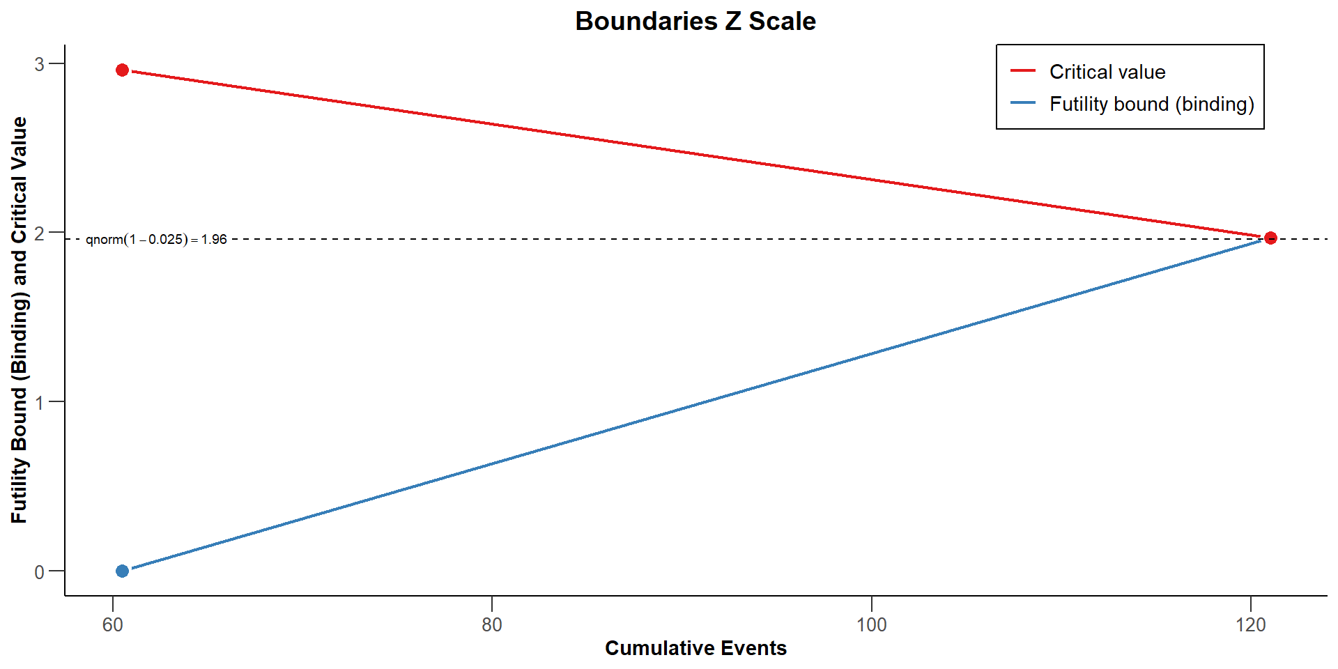


$`Boundaries Effect Scale`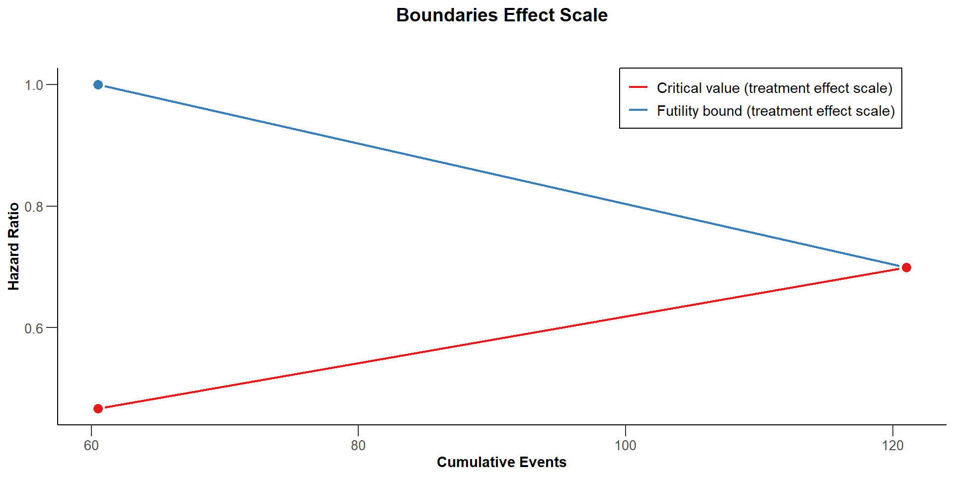


$`Boundaries p Values Scale`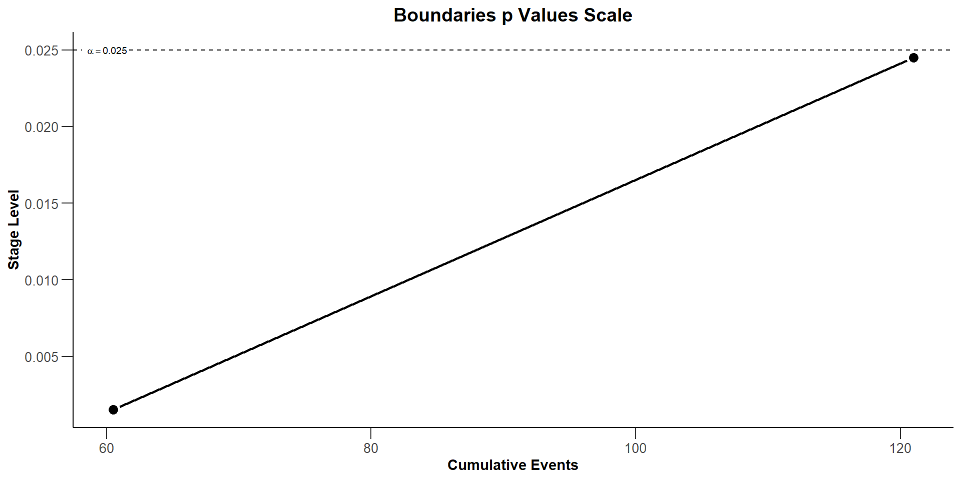


$`Error Spending`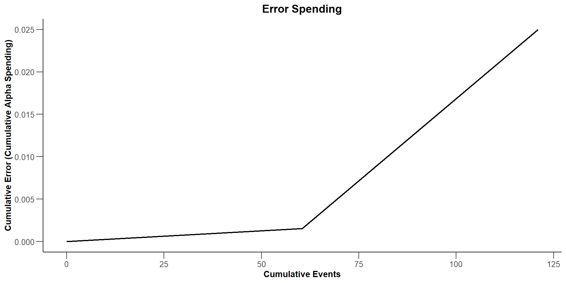


$`Overall Power and Early Stopping`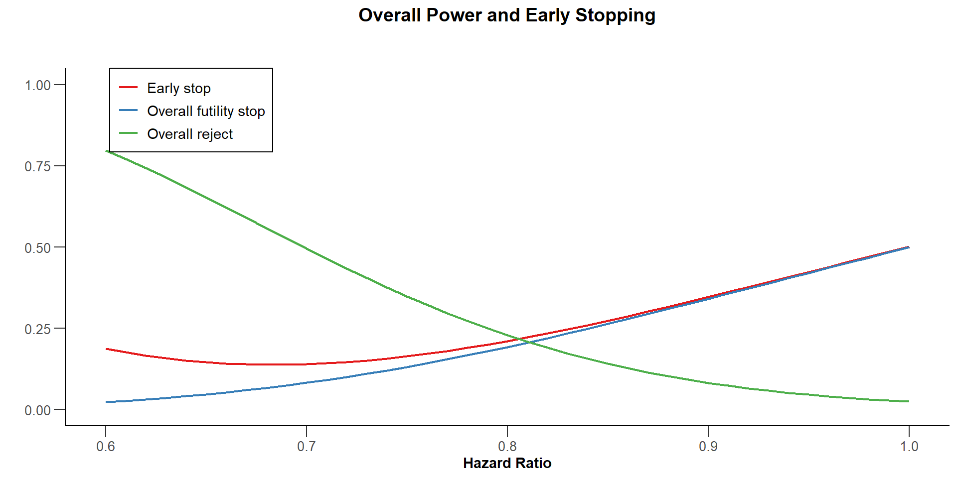


$`Number of Events`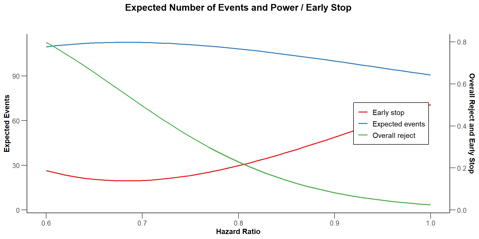


$`Overall Power`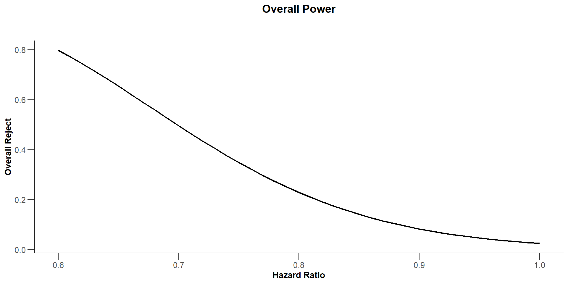


$`Overall Early Stopping`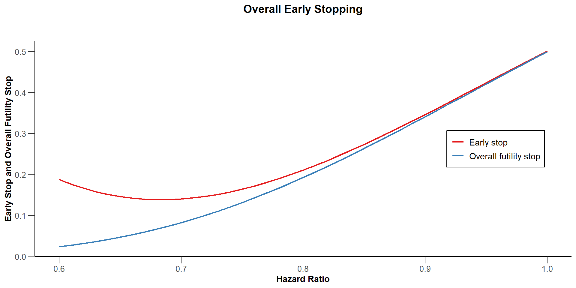


$`Expected Number of Events`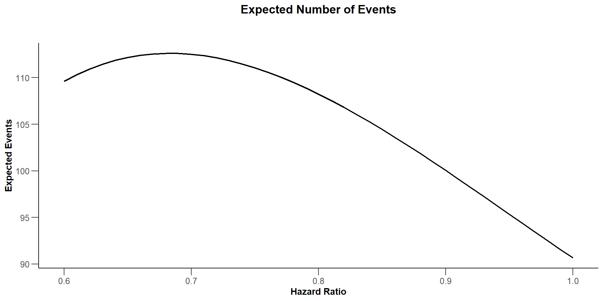


$`Study Duration`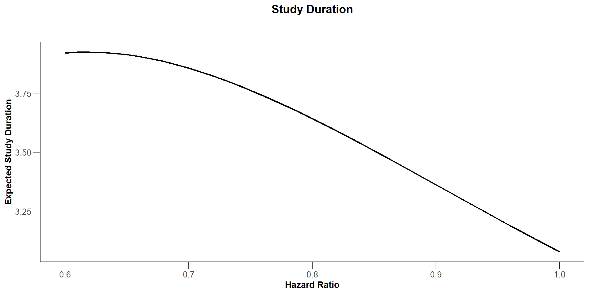


$`Expected Number of Subjects`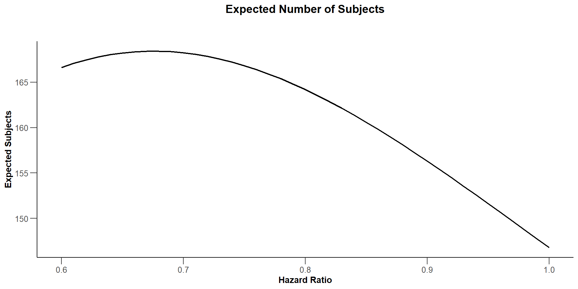


$`Analysis Time`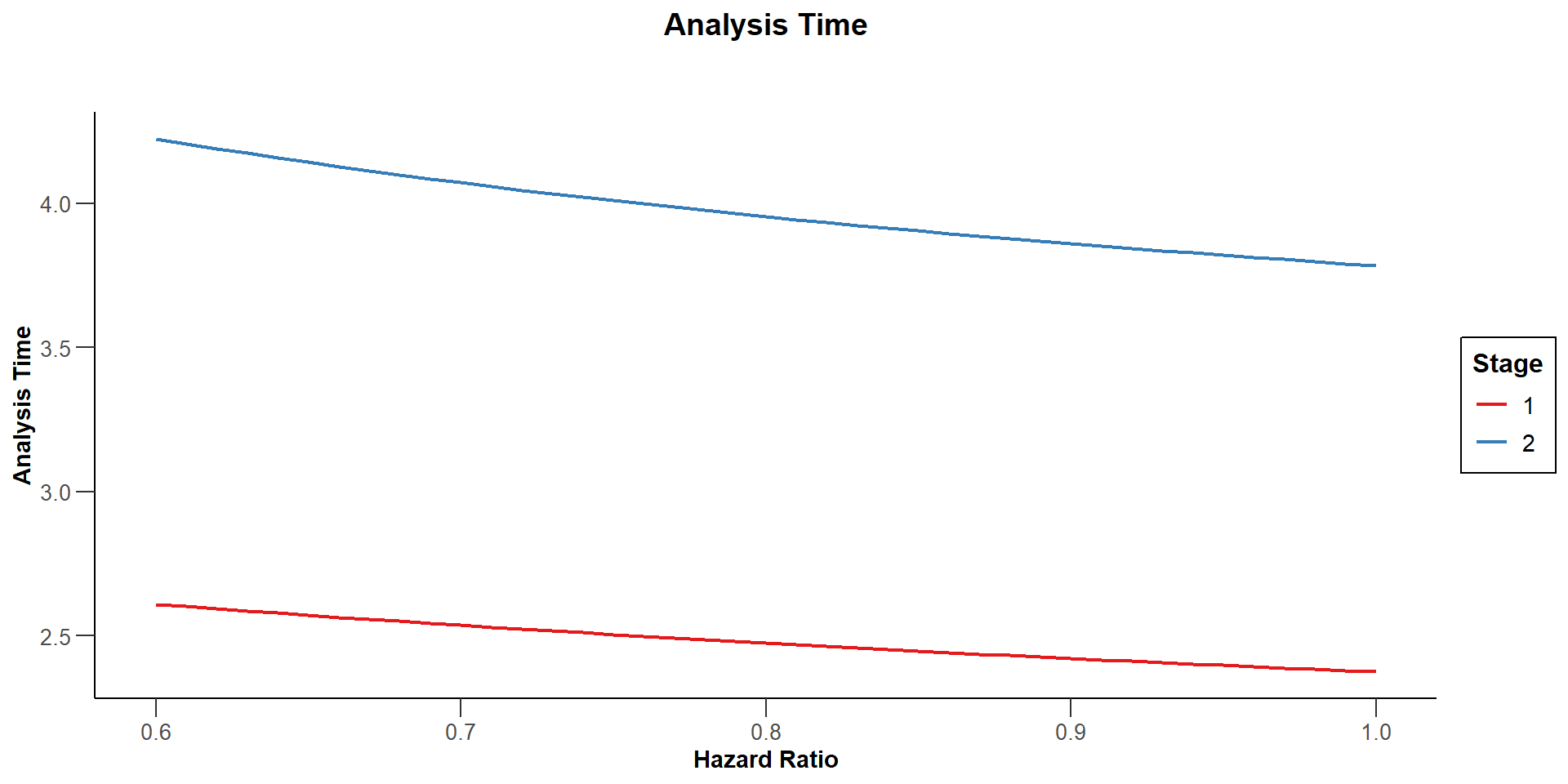


$`Cumulative Distribution Function`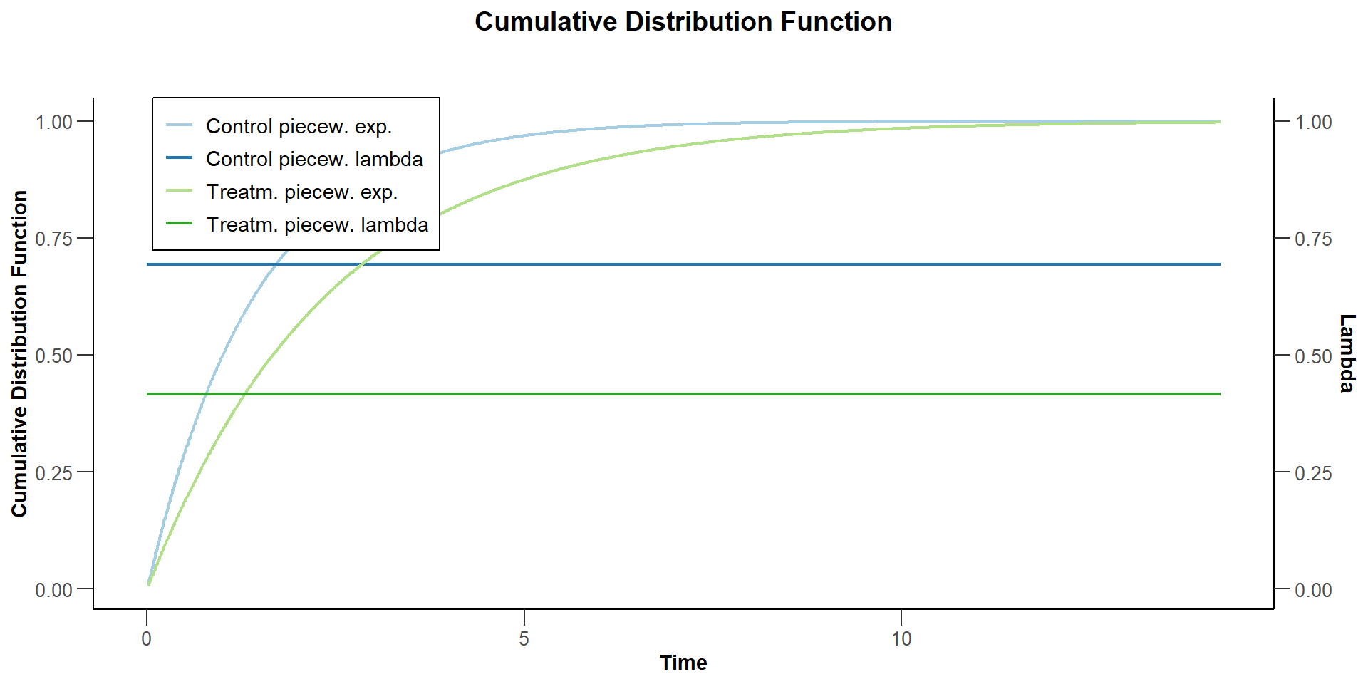


$`Survival Function`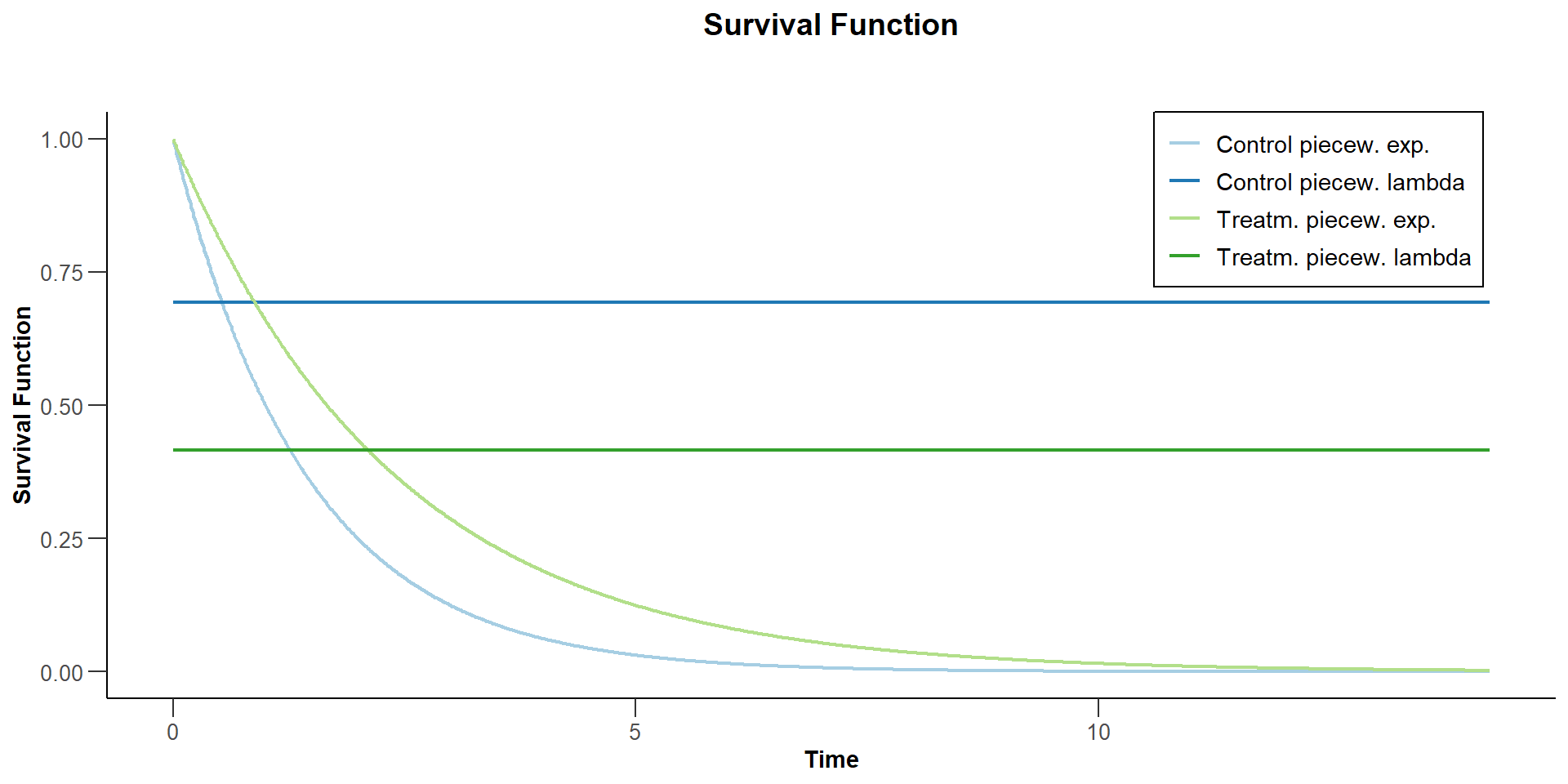

Survival Analysis

Interim Analysis Stage

Suppose at the interim analysis, the observed number of events is 67 and the value of the Z-statistic is -1.10 (where negative values correspond to treatment benefit).

Question 7

Re-calculate the stopping boundary based on the observed 67 events at the interim analysis.

Assume the same alpha-spending function as above.
Assume the planned maximum number of events is 121.

getDesignGroupSequential(
  typeOfDesign = "asOF", 
  informationRates = c(67 / 121, 1),             
  alpha = 0.025
) |> fetch(criticalValues)

$criticalValues
[1] 2.795107 1.974428

What is the interim analysis decision?

Test decision

Continue to the next stage, since the Z statistic is between 0 (futility bound) and -2.795 (efficacy bound)

\(\hspace{2cm}\)

Direction of test statistic

NOTE: The function getDesignGroupSequential() doesn’t know which direction of Z statistic indicates treatment benefit. By default, the critical values are displayed assuming positive Z is beneficial.

Final Analysis Stage

Suppose at the final analysis, the observed number of events is 129 and the value of the Z-statistic is -2.00 (where negative values correspond to treatment benefit).

Question 8

Re-calculate the stopping boundary based on the observed 67 events at interim and 129 events at the final analysis.

Since we have deviated from the planned maximum number of events (= 121), our actual alpha spent no longer follows the O’Brien-Fleming-type alpha-spending function. Use the argument typeOfDesign = "asUser" instead.

getDesignGroupSequential(
  typeOfDesign = "asOF", 
  informationRates = c(67 / 121, 1),             
  alpha = 0.025
) |> fetch(alphaSpent)

$alphaSpent
[1] 0.002594128 0.024999990

getDesignGroupSequential(
    typeOfDesign = "asUser", 
    userAlphaSpending = c(0.0025941, 0.025),
    informationRates = c(67 / 129, 1),             
    alpha = 0.025
) |> fetch(criticalValues)

$criticalValues
[1] 2.795110 1.976408

Final test decision

Reject the null hypothesis since Z < -1.9764

Alternative

Use maxInformation and getAnalysisResults()

# Dummy design
designDummy <- getDesignGroupSequential(
    typeOfDesign = "asOF",
    directionUpper = FALSE
)
dataExample <- getDataset(
    cumEvents = 67,
    cumLogRanks = c(-1.10)
)
getAnalysisResults(
    design = designDummy, 
    dataInput = dataExample, 
    maxInformation = 121
) |> summary()

Analysis results for a survival endpoint

Sequential analysis with 2 looks (group sequential design), one-sided overall significance level 2.5%. The results were calculated using a two-sample logrank test. H0: hazard ratio = 1 against H1: hazard ratio < 1.

Stage	1	2
Planned information rate	55.4%	100%
Cumulative alpha spent	0.0026	0.0250
Stage levels (one-sided)	0.0026	0.0242
Efficacy boundary (z-value scale)	2.795	1.974
Cumulative effect size	0.764
Overall test statistic	-1.100
Overall p-value	0.1357
Test action	continue
Conditional rejection probability	0.0418
95% repeated confidence interval	[0.386; 1.513]
Repeated p-value	0.2669

Second stage

dataExample <- getDataset(
    cumEvents = c(67, 129),
    cumLogRanks = c(-1.10, -2.0)
)
getAnalysisResults(
    design = designDummy, 
    dataInput = dataExample, 
    maxInformation = 121
) |> summary()

Analysis results for a survival endpoint

Stage	1	2
Planned information rate	51.9%	100%
Cumulative alpha spent	0.0026	0.0250
Stage levels (one-sided)	0.0026	0.0241
Efficacy boundary (z-value scale)	2.795	1.976
Cumulative effect size	0.764	0.703
Overall test statistic	-1.100	-2.000
Overall p-value	0.1357	0.0228
Test action	continue	reject
Conditional rejection probability	0.0439
95% repeated confidence interval	[0.386; 1.513]	[0.496; 0.996]
Repeated p-value	0.2669
Final p-value		0.0237
Final confidence interval		[0.498; 0.996]
Median unbiased estimate		0.704

Extensions

Drop-outs

Question 9

Going back to the assumptions in Question 3, what is the expected study duration for a fixed sample size design if we specify in addition that 2% of subjects on each arm will drop out per year?

Was 4.776 without dropouts

getSampleSizeSurvival(
    alpha = 0.025, 
    beta = 0.2, 
    hazardRatio = 0.6, 
    median2 = 1, 
    accrualTime = c(0, 3),
    accrualIntensity = 50,
    dropoutRate1 = 0.02, 
    dropoutRate2 = 0.02, 
    dropoutTime = 1,
    allocationRatioPlanned = 1
) |> fetch(studyDuration)

studyDuration 
     4.984452

Staggered Patient Entry

Question 10

Suppose the patient entry is not uniform, but staggered in intervals. For example, the accrual starts with 30 patients in the first year, 40 in the second, and 50 in the third.

What is the expected study duration (under H1)?

Was 4.984 with uniform patient entry

Note

We have to increase the accrual time because otherwise #events > #patients

getSampleSizeSurvival(
    alpha = 0.025, 
    beta = 0.2, 
    median2 = 1, 
    hazardRatio = 0.6, 
    accrualTime = c(0, 1, 2, 3.5),
    accrualIntensity = c(30, 40, 50),
    dropoutRate1 = 0.02, 
    dropoutRate2 = 0.02, 
    dropoutTime = 1,
    allocationRatioPlanned = 1
) |> summary()

Sample size calculation for a survival endpoint

Fixed sample analysis, one-sided significance level 2.5%, power 80%. The results were calculated for a two-sample logrank test, H0: hazard ratio = 1, H1: hazard ratio = 0.6, control median(2) = 1, accrual time = c(1, 2, 3.5), accrual intensity = c(30, 40, 50), dropout rate(1) = 0.02, dropout rate(2) = 0.02, dropout time = 1.

Stage	Fixed
Stage level (one-sided)	0.0250
Efficacy boundary (z-value scale)	1.960
Efficacy boundary (t)	0.700
Number of subjects	145.0
Number of events	120.3
Analysis time	5.83
Expected study duration under H1	5.83

Legend:

(t): treatment effect scale

More Complicated Survival Distributions

Suppose now that the control arm follows a piecewise exponential distribution. For the first year the hazard rate is log(2) / 1 = 0.693, and thereafter the hazard rate is 0.5.

Question 11

What is the expected study duration?

Was 5.83 with constant hazard rate

getSampleSizeSurvival(
    alpha = 0.025, 
    beta = 0.2, 
    piecewiseSurvivalTime = c(0, 1), 
    lambda2 = c(0.693, 0.5), 
    hazardRatio = 0.6,
    accrualTime = c(0, 1, 2, 3.5),
    accrualIntensity = c(30, 40, 50),
    dropoutRate1 = 0.02, 
    dropoutRate2 = 0.02, 
    dropoutTime = 1
) |> fetch(studyDuration)

studyDuration 
     6.864769

Non-Proportional Hazards

Suppose that, in addition to the changing hazard rate on the control arm, the hazard ratio also changes.

Suppose that the hazard ratio during the first year is 0.6. Thereafter, the hazard ratio is 0.8.

Question 11

Use the function getSimulationSurvival() to calculate the power of the fixed sample size design with 3.5 years recruitment (50 subjects per year).

tictoc::tic()
getSimulationSurvival(
    piecewiseSurvivalTime = c(0, 1), 
    lambda2 = c(0.693, 0.5), 
    hazardRatio = c(0.6, 0.8),
    directionUpper = FALSE, 
    plannedEvents = 121,
    accrualTime = c(0, 3.5), 
    accrualIntensity = 50,
    maxNumberOfIterations = 10000
) |> fetch(overallReject)

overallReject 
       0.5766

tictoc::toc()

0.8 sec elapsed

Summary

Introduction to design and analysis of survival design
For survival designs, many additional options for specifying patient recruitment, survival time distribution, and effect size pattern available
Flexible trial conduct through use of \(\alpha\)-spending approach
Caveat: No data-driven reassessment of information possible without jeopardizing Type I error control
Alternative: p-value combination approach: use of inverse normal combination of Fisher’s combination test
Application, e.g., within promizing zone design, see Vignette Promizing Zone Design with rpact
Use of fast and flexible getSimulationSurvival() function for assessing these designs

RPACT Survival Designs

RPACT Survival Designs

The Situation

Required Number of Events

Required Number Of Subjects

Required Number Of Subjects

Adding An Interim Analysis

Adding An Interim Analysis

Adding A Futility Boundary

Survival Analysis

Interim Analysis Stage

Final Analysis Stage

Alternative

Extensions

Drop-outs

Staggered Patient Entry

More Complicated Survival Distributions

Non-Proportional Hazards

Summary

Questions??